Vnano | Solve The Lorenz Equations Numerically

A program to solve the Lorenz equations (see Theoretical Model section for details) numerically by using the Runge-Kutta 4th order (RK4) method, and output data to plot the solution curve on a 3D graph. The plotted solution curve is well-known as the "Lorenz Attractor"

Code of this script is written in the Vnano. Code written in C, C++, and Java® are also distributed in Code section. In addition, the Vnano is a subset of the VCSSL, so you can execute this script as VCSSL code, with changing the extention of the script file to ".vcssl" .

�X�|���T�[�����N

---

How to Use

Download and Extract

At first, click the "Download" button at the above of the title of this page by your PC (not smartphone). A ZIP file will be downloaded.

Then, please extract the ZIP file. On general environment (Windows®, major Linux distributions, etc.), you can extract the ZIP file by selecting "Extract All" and so on from right-clicking menu.

» If the extraction of the downloaded ZIP file is stopped with security warning messages...

Execute this Program

Next, open the extracted folder and execute this VCSSL program.

For Windows

Double-click the following batch file to execute:

For Linux, etc.

Execute "VCSSL.jar" on the command-line terminal as follows:

» If the error message about non-availability of "java" command is output...

Output Data For Plotting A Graph, And Save The Content to A File

Output Data For Plotting A Graph

When the program has started, a window will be displayed, and data for plotting a graph will be printed on the window line by line:

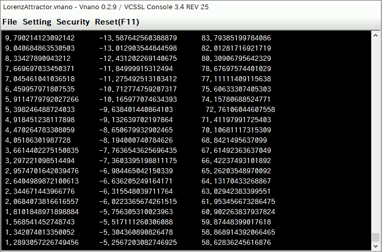
In printed data, coodinate values (x,y,z) of each point are described as "x    y    z" in a line, so each line represents each point to be plotted.

When the calculation has completed, printing of data stops (by default setting, it will complete immediately).

Save Data to A File

To save the printed data to a file, choose "File" > "Save File ..." menu, from the menubar at the top of the window.

See also: How to Plot Graphs section, which guides how to plot a graph from printed/saved data, and explains what is plotted in the graph.

How to Plot Graphs

When You Are Executing This Program on The VCSSL Runtime (Downloaded From This Page)

If you are executing this program as explained in How to Use section, it is executed by software "VCSSL Runtime", which is bundled in the downloaded package.

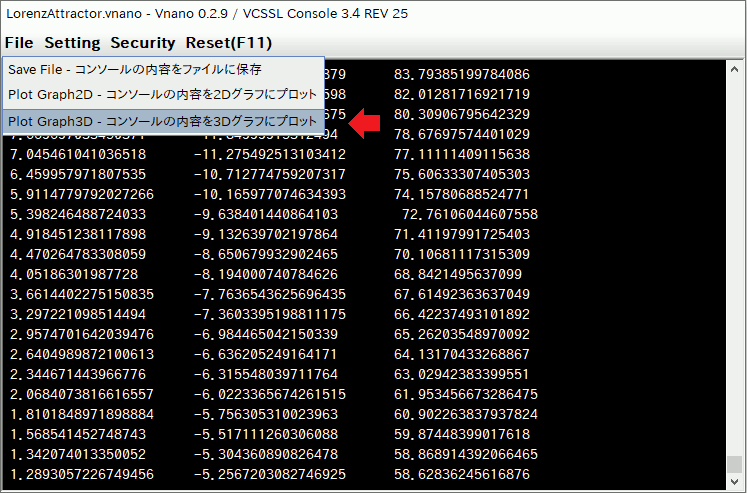
On the VCSSL Runtime, 2D & 3D graph plotting features are available by default, so you can plot printed data to a graph very easily. Let's plot it. After when the calculation has completed, choose "File" > "Plot Graph3D ..." menu, from the menubar at the top of the window:

Then, printed data on the window will plotted to a graph. By default, data will be plotted by only points, so enable "With Lines" option, from the menu bar of the graph window. Then all points on the graph will be connected by lines as the follows:

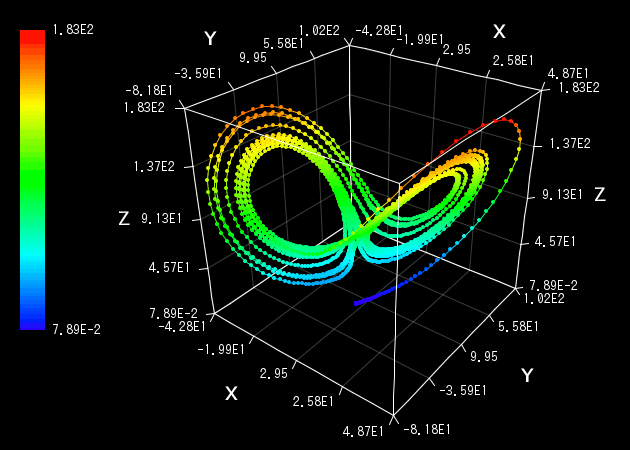
The above graph represents the solution curve of Lorenz equations, solved numerically by using Runge-Kutta 4th order (RK4) method.

If you want to play the animation drawing the solution curve from the beginning point to the end, click "Tool" > "Animation" menu, from the menu bar of the graph window.

An example of the animation is here (6.5 MB).

When You Are Using The RINPn (A Scientific Calculator Software)

The RINPn, a scientific calculator software, can execute programs written in the Vnano (containing this program), but graph plotting features are not supported by default.

Hence, it is necessary to use the RINPn with an independent graph plotting software, for plotting graphs from calculated data. The content of output data of this program is described in a standard format, so it is available on various graph plotting software, e.g.: gnuplot.

Let's plot the graph practically. We use "RINEARN Graph 3D", which is a 3D graph plotting software developped by the RINEARN, as same as the RINPn, the Vnano, and so on. You can get the RINEARN Graph 3D in free, from the following website:

RINEARN Graph 3D   Official Website

https://www.rinearn.com/en-us/graph3d/

When the RINEARN Graph 3D is executed, a graph window will be displayed. The graph window of the RINEARN Graph 3D is completely the same as it of the VCSSL Runtime (we saw it in the previous section), because the graph-plotting feature of the VCSSL Runtime uses the RINEARN Graph internally.

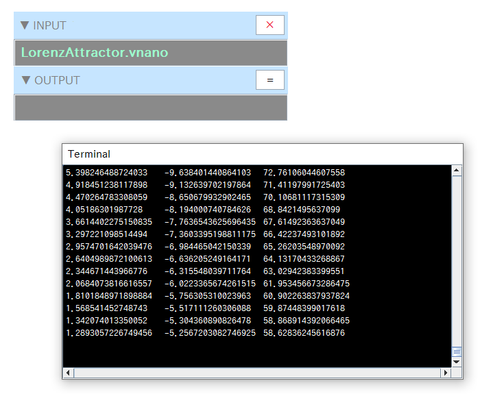
By using the RINEARN Graph 3D, you can plot a graph from output data of this program very easily. At first, execute this program on the RINPn: Put this program in the folder of the RINPn, and input the file name of the program "IntegralForPlot.vnano", and press Enter key. Then a window will be displayed, and calculated data will be printed on the window line by line:

Next, select all lines of data on the above window (you can do it by pressing "Ctrl" + "A" keys), and copy it to the clipboard from the right-click menu, and paste it on the RINEARN Graph 3D from the right-click menu. Then the pasted data will be plotted on the graph window:

As the above, we can plot the completely same graph as the VCSSL Runtime.

When You Are Using The RINPn on The Command-Line Terminal

It is helpful to register pathes of "bin" folders of the RINPn and the RINEARN Graph 3D to the environment variable "PATH" or "Path" of your OS. Then you can use RINPn and the RINEARN Graph 3D on the command-line terminal, as "rinpn" and "ring3d" commands, as follows:

When above command-lines are executed, calculated data will be saved as a file "data.txt", and a graph will be plotted from data in "data.txt" (the graph will be displayed on a window).

When You Want to Use The Gnuplot For Plotting Graphs

Also, if you want to plot a graph by using the gnuplot, input as follows:

and so on, where "splot ... with lp" means that we want to plot a graph with lines(l) and points(p), "pt 7" is for specifying the type of points (markers) to filled circles (the number may depend on your environment and the version of the gnuplot), "ps 0.5" is for specifying the size of points. "palette" is for using gradation colors to render the graph.

The displayed graph on the gnuplot is:

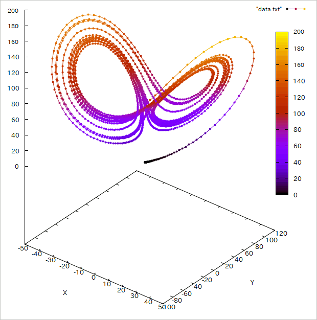
As the above, we can plot graphs from output data of this program on various graph-plotting software.

---

�X�|���T�[�����N

---

Theoretical Model

As shown above, this program solves Lorenz equations numerically, and output data for plotting the solution curve on a graph. In this section, we describe some background knowledge about Lorenz equations and its solutions.

The Lorenz Equation

The Lorenz equations is the following non-linear differential equation(s):

\[ \frac{dx}{dt} = - \sigma x + \sigma y \] \[ \frac{dy}{dt} = - x z + \rho x + y \] \[ \frac{dz}{dt} = x y - \beta z \]

Above equations firstly appeared in this paper (Accessible on the website of the American Meteorological Society), published in 1963. The author is Edward Norton Lorenz, an American meteorologist, researched at MIT.

There is a page for Lorenz equations on the Wikipedia, so see it if you want to grasp behaviour of the equation briefly.

The Solution Curve

As the above, the Lorenz equations give time-derivatives of x/y/z coordinates. In other words, they give the rule that how a point at \((x,y,z)\) moves at each moment. So, Let's put a point at \((x_0,y_0,z_0)\), where \(x_0,y_0,z_0\) are referred to as "initial values". Then the point starts to move. At each moment, the speed and the direction of the movement of the point are determined by the velocity vector \( \left( \frac{dx}{dt},\frac{dy}{dt},\frac{dz}{dt} \right) \), and its values are determined by the Lorenz equations. The following is the animation of the movement of the point:

As the above animation, behaviour of a point under the Lorenz equations are non-periodic. The point whimsically jumps between two rings, under some conditions. Then the trajectory of the movement of the point, referred to as "the solution curve" (because the movement of the point satisfies lorenz equations), takes butterfly-like shape as the following figure:

This butterfly-like structure is well-known as the "Lorenz Attractor", which is a kind of attractor.

Sensitivity to Initial Conditions

Let's compare movements of two points (red and green) under the Lorenz equations, where points are put very close position at the beginning:

As the above animation, distance between points grows as time proceeds, and movements and locations of points after some time elapsed are completely different from each other.

The above is cause by that movements under the Lorenz equations exhibit the "sensitivity to initial conditions". Generally, on systems exhibit such sensitivity, distance between two close points grows exponentially as time proceeds. Hence, if two initial point are not the completely same, no matter how they are closer initially, trajectories will completely separate after some time elapsed.

Hard to Predict

As shown above, behaviour under the Lorenz equations is non-periodic and whimsical (even though it is completely deterministic), and has the sensitivity to initial conditions.

The above means that, when we want to predict the future of behaviour under the Lorenz equations, we are required to calculate movements of a point in complete precision at every moment. In addition, we must set the initial values in complete precision, even if they are irrational numbers. If any small error exists somewhere in the above, it grows exponentially as time proceeds, and the prediction will be completely broken, after some (not so long) time elapsed.

In addition, unfortunately, we can not get analytical general solutions of Lorenz equations, so we are required to compute numerical solutions by running programs on computers, as we performed in this page. However, generally, computers handle real numbers in some limited (incomplete) precision, so tiny numerical errors will be contained in calculation results between real numbers. Also, on the computer, we compute behaviour of a point at discrete time, so discretization errors will be contained in calculation results at each time.

Therefore, it is very hard - almost impossible - to predict the far future of behaviour of a point under the Lorenz equations in good precision.

The same is true for other "chaotic" systems. Behaviour under the Lorenz equations (Lorenz system) is a very simple example of chaotic systems. If you interested in this kind of problem, search webpages/books of Chaos theory, Butterfly effect, and so on. Then you might grasp why the very-long-range weather prediction is difficult, as Edward Norton Lorenz said in his paper.

Code

Entier Code

Code of this program is written in the Vnano. The Vnano has a simple C-like syntax, so if you accustomed with C or C-like programming languages, you probably can read/customize the content of code easily.

The following is the entier code:

Please feel free to ask me if you have any questions!

License

The license of this VCSSL / Vnano code (the file with the extension ".vcssl" / ".vnano") is CC0 (Public Domain), so you can customize / divert / redistribute this VCSSL code freely.

Also, if example code written in C/C++/Java are displayed/distributed on Code section of this page, they also are distributed under CC0, unless otherwise noted.