Now Loading...

Please download on PC (not smartphone) and extract the ZIP file. Then double-click VCSSL.bat (batch file) to execute for Microsoft® Windows®, or execute VCSSL.jar (JAR file) on the command line for Linux® and other OSes.
For details, see How to Use.

Vnano | Output Data of Numerical Integration For Plotting Graph

A program to perform an integration numerically, and output data for plotting the integrated function (the function of the indefinite integral with the lower limit (basepoint) A) into a graph. How to plot graphs practically is also explained in this article.

Code of this script is written in the Vnano. Code written in C, C++, and Java® are also distributed in Code section. In addition, the Vnano is a subset of the VCSSL, so you can execute this script as VCSSL code, with changing the extention of the script file to ".vcssl" (In such case, please enable the "import" statement at the near the top of the code, which is commented-out by default).

Also, this program is an modified version of previous article's program, so please see the previous article for details of algorithms of numerical integrations.

�X�|���T�[�����N

How to Use

Download and Extract

At first, click the "Download" button at the above of the title of this page by your PC (not smartphone). A ZIP file will be downloaded.

Then, please extract the ZIP file. On general environment (Windows®, major Linux distributions, etc.), you can extract the ZIP file by selecting "Extract All" and so on from right-clicking menu.

» If the extraction of the downloaded ZIP file is stopped with security warning messages...

Execute this Program

Next, open the extracted folder and execute this VCSSL program.

For Windows

Double-click the following batch file to execute:

For Linux, etc.

Execute "VCSSL.jar" on the command-line terminal as follows:

» If the error message about non-availability of "java" command is output...

Output Data For Plotting A Graph, And Save The Content to A File

Output Data For Plotting A Graph

When the program has started, a window will be displayed, and data for plotting a graph will be printed on the window line by line:

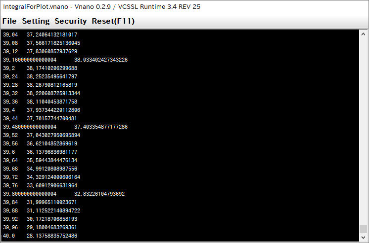
In printed data, coodinate values (x,y) of each point are described as "x    y" in a line, so each line represents each point to be plotted.

When the calculation has completed, printing of data stops (by default setting, it will complete immediately).

Save Data to A File

To save the printed data to a file, choose "File" > "Save File ..." menu, from the menubar at the top of the window.

See also: How to Plot Graphs section, which guides how to plot a graph from printed/saved data, and explains what is plotted in the graph.

How to Change the Integrant Function, Interval, etc.

For changing the integrant function, modify the content of the function "f(x)" defined in the script. For changing the interval of the integration, modify values of variables "A" and "B" in the script. In addition, if necessary, modify the value of the variable "N" in the script, which is the number of tiny intervals (See: Code section).

By default settings, "cos(x)" will be integrated from x = 0 to x = 1.

How to Change The Number of Lines in Output Data (The Number of Points Plotted on A Graph)

For controling the number of lines in output data, which equal to the number of plotted points on a graph, modify the value of variable PRINT_POINTS in code.

Please note that, the actual number of plotted points will be different from the value of PRINT_POINTS, in some extent. » Why?

How to Change The Algorithm of The Integration

In this script, as algorithms of the numerical integration, you can use the rectangular method, the trapezoidal method, and the Simpson's rule. Each algorithm is implemented as a line in the script (See: Code section), so please add/remove "//" (a line starts with "//" will be ignored) at those lines, for selecting the algorithm you want to use. By default, the Simpson's rule will be used.

How to Plot Graphs

When You Are Executing This Program on The VCSSL Runtime (Downloaded From This Page)

If you are executing this program as explained in How to Use section, it is executed by software "VCSSL Runtime", which is bundled in the downloaded package.

On the VCSSL Runtime, 2D & 3D graph plotting features are available by default, so you can plot printed data to a graph very easily. Let's plot it. After when the calculation has completed, choose "File" > "Plot Graph2D ..." menu, from the menubar at the top of the window:

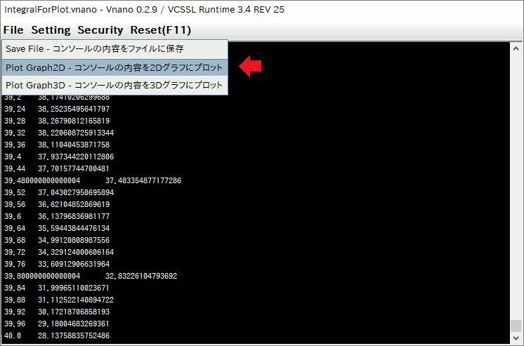
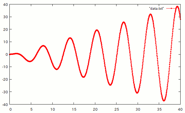
Then, printed data on the window will plotted to a graph:

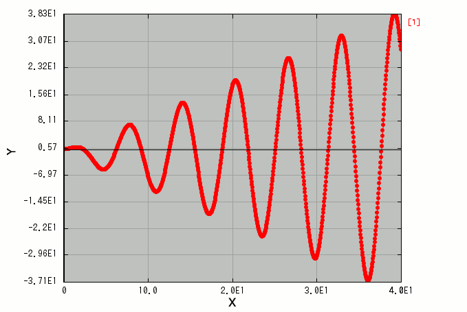
On the above graph, the y-coordinate value of each point represents the numerically integrated value of the integrant function f(x), from the lower limit A (= 0) to the x-coordinate value of the point. In a word, the plotted line represents the function of the indefinite integral with the lower limit (basepoint) A:

\[ F(x) = \int^x_A f(t) dt \]

Data plotted on the above graph was calculated under the default settings, f(x) = cos(x) and A = 0, so the theoretically correct expression of F(x) is:

\[ F(x) = \int^x_0 t \cos t dt = \big[ t \sin t + \cos t \big]^x_0 = x \sin x + \cos x + 1 \]

The above graph maches very well* with the above theoretical expression of F(x).

When You Are Using The RINPn (A Scientific Calculator Software)

The RINPn, a scientific calculator software, can execute programs written in the Vnano (containing this program), but graph plotting features are not supported by default.

Hence, it is necessary to use the RINPn with an independent graph plotting software, for plotting graphs from calculated data. The content of output data of this program is described in a standard format, so it is available on various graph plotting software, e.g.: gnuplot.

Let's plot the graph practically. We use "RINEARN Graph 2D", which is a 2D graph plotting software developped by the RINEARN, as same as the RINPn, the Vnano, and so on. You can get the RINEARN Graph 2D in free, from the following website:

RINEARN Graph 2D   Official Website

https://www.rinearn.com/en-us/graph2d/

When the RINEARN Graph 2D is executed, a graph window will be displayed. The graph window of the RINEARN Graph 2D is completely the same as it of the VCSSL Runtime (we saw it in the previous section), because the graph-plotting feature of the VCSSL Runtime uses the RINEARN Graph internally.

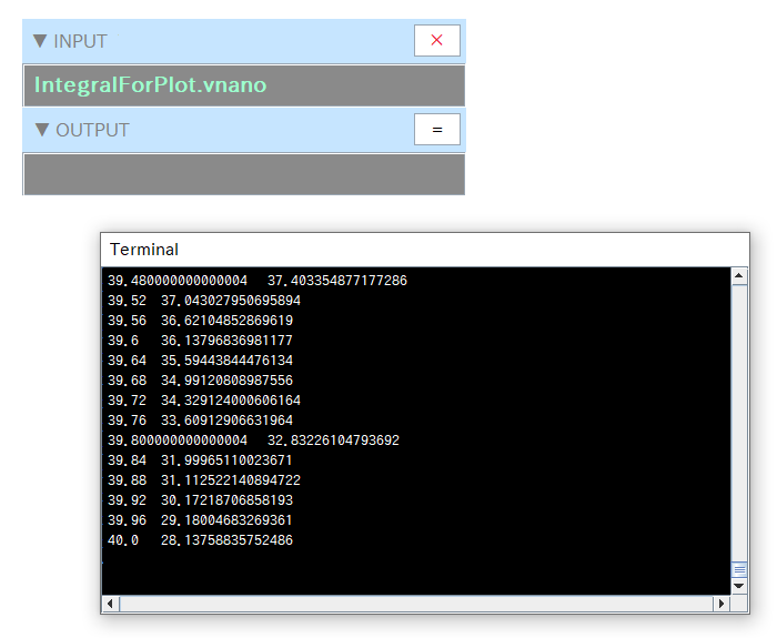
By using the RINEARN Graph 2D, you can plot a graph from output data of this program very easily. At first, execute this program on the RINPn: Put this program in the folder of the RINPn, and input the file name of the program "IntegralForPlot.vnano", and press Enter key. Then a window will be displayed, and calculated data will be printed on the window line by line:

Next, select all lines of data on the above window (you can do it by pressing "Ctrl" + "A" keys), and copy it to the clipboard from the right-click menu, and paste it on the RINEARN Graph 2D from the right-click menu. Then the pasted data will be plotted on the graph window:

As the above, we can plot the completely same graph as the VCSSL Runtime.

When You Are Using The RINPn on The Command-Line Terminal

It is helpful to register pathes of "bin" folders of the RINPn and the RINEARN Graph 2D to the environment variable "PATH" or "Path" of your OS. Then you can use RINPn and the RINEARN Graph 2D on the command-line terminal, as "rinpn" and "ring2d" commands, as follows:

When above command-lines are executed, calculated data will be saved as a file "data.txt", and a graph will be plotted from data in "data.txt" (the graph will be displayed on a window).

When You Want to Use The Gnuplot For Plotting Graphs

Also, if you want to plot a graph by using the gnuplot, input as follows:

and so on, where "with lp" means that we want to plot a graph with lines(l) and points(p), "pt 7" is for specifying the type of points (markers) to filled circles (the number may depend on your environment and the version of the gnuplot), "ps 0.5" is for specifying the size of points.

The displayed graph on the gnuplot is:

As the above, we can plot graphs from output data of this program on various graph-plotting software.

�X�|���T�[�����N

Code

Entier Code

Code of this program is written in the Vnano. The Vnano has a simple C-like syntax, so if you accustomed with C or C-like programming languages, you probably can read/customize the content of code easily.

Let's see the entier code:

This program is an modified version of previous article's program, so please see the previous article for details of algorithms of numerical integrations (the rectangular method, the trapezoidal method, and the Simpson's rule). Here we omit explanation of such algorithmic aspects, and forcus on: how/when this program outputs what values?

The Top of Code

Code starts with the following content:

The first line "coding ..." is for declaring the text-encoding of the script file, for preventing encoding/decoding-related probrems (e.g.: "mojibake").

The next line "import ..." (which is used for loading a library) is necessary if you execute this script as VCSSL code, but it is not necessary when you exeute this script as Vnano code, so it is commented-out by default.

Definitions of The Integrant Function, The Interval of The Integration, etc.

In the next part, the integrant function, the interval of the integration, and so on are defined:

When you want to customize settings of the integration, modify the above code. Basically, define the integrant function as the function "f(x)" in the above code, and input the value of the lower/upper-limit of the integration to the variable "A" / "B".

"N" represents the number of tiny intervals (for details, see the latter sections). When you make the value of N larger, the precision of the integrated value basically increses, but required time for the calculation become longer. Please note that, if you set the immediately large value to N, the precision might decrease, because the number of total cycles of the integration loop become very large, so tiny numerical errors affect many times to the result.

Setting Parameters for Outputting Data (for Plotting Graphs)

Then, setting parameters for outputting data are defined:

This part does not exist in the previous article's program. As commented in code, to the value of the variable "PRINT_POINTS", set the number of points you want to plot on the graph. Please note that, the actual number of plotted points will be different from the value of PRINT_POINTS, in some extent.

The Core Part: The Loop Performing The Numerical Integration and Outputting Data

The next is the core part of this program: the loop for calculating the value of integral numerically, with outputting data:

For details of numerical integration algorithmis used in this program (the rectangular method, the trapezoidal method, and the Simpson's rule), see the previous article.

To put it briefly, here this program approximately calculates area between the integrant function f(x) and the x-axis, in the range from A to B (which equals to the integrated value of  f(x) from A to B). In most simple way, split the interfal from A to B into N-"tiny interval"s, and approximate area of each tiny interval as rectangle, and calculate the summation value of all rectangles (in the for-loop):

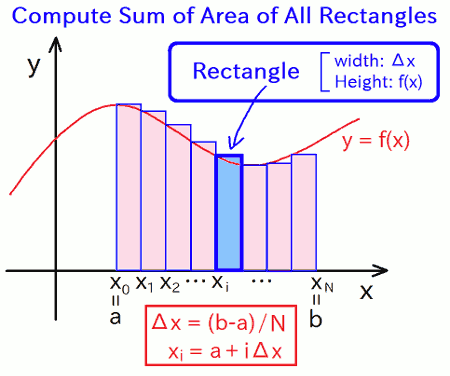
The rectangular method approximates area of each tiny interval as a rectangle, the trapezoidal method approximates area of each tiny interval as a trapezoid, and the Simpson's rule approximates the upper curve of area of each interval by using a quadratic function. In the previous article, we focused on that how precisions of result (numerical integralation) values improves drastically by switching algorithms.

On the other hand, in the previous article, we had not interested in how the intagration (intermediate) value changes on the way from A to B. We focuse on it in this article. Hence, we output the intermediate value of the variable "value" to which area of tiny interval are integrated, periodically in the for-loop of the numerical integration:

An (intermediate) integration value is printed at the line-45. It prints a data-line of which content is "x    value", where the "x" is the x-coordinate value on the way from A to B, and "value" is the value of the variable to which area of tiny interval are integrated, which equals to the numerically (approximately) calculated value of the integral of  f(x) from A to "x":

\[ F(x) = \int^x_A f(t) dt \]

On the graph, the above data-line will be plotted as a point at (x,y) = ("x", "value"). This program prints the above data-line periodically in the for-loop, with changing the value of "x" little by little from A to B. Therefore, many points are plotted on (x,y) = (x,F(x)), so we can draw the graph of F(x) approximately.

The Last Part Outputting The Last Value of The Integration

By the way, as shown in the previous section, values of variables "x" and "value" are printed at the top in the for-loop. This means that, "the x-coordinate value at the left-bottom point of the i-th tiny interval" and "the integration value just before adding area of i-th interval" are printed together in a data-line.

The above way (especially the part "before adding...") might seem to be a little strange. Actually, it may be incorrect if you want to check the integration value from 0-th to i-th intervals for debugging and so on. However, it is correct for our current purpose: print the values of (xi, F(xi)); where xi is the x-coordinate value of the left-bottom point of the i-th tiny interval, and the value of F(xi) is given approximately as the summation value of area of all tiny intervals locating at the left-side of the line x = xi. The i-th tiny interval locates at the right-side of the line x = xi, so its area should not be added to the value of F(xi). This is the reason of why we print the integration value just before adding area of i-th tiny interval, with the value of xi.

However, in the above way, there is a pitfall that: we can't output the integration value F(x) at x = B (the upper limit), because it is the integration value after adding area of the last tiny interval. Hence, when all cycles of the for-loop has completed, this program prints the integration value which gives the approximate value of F(B), as follows:

Due to the above code, we can get the integration value from A to B by reading the last value in the right-column of output data, so you can use this program for the same purpose as the previous article's program.

License

The license of this VCSSL / Vnano code (the file with the extension ".vcssl" / ".vnano") is CC0 (Public Domain), so you can customize / divert / redistribute this VCSSL code freely.

Also, if example code written in C/C++/Java are displayed/distributed on Code section of this page, they also are distributed under CC0, unless otherwise noted.