Circular Wave Animation

This is a VCSSL program that animates circular waves propagating across a plane, based on parameters such as amplitude, wavelength, and period.

In the previous article and the one before that, we visualized sine waves propagating along a line -- in other words, on a one-dimensional medium.

This time, we'll extend the idea to two-dimensional media and look at waves that spread out over a surface. Specifically, we'll animate circular waves that radiate outward in concentric circles from a central source.

[ Related Article ]

• Previous: Wave Interference Animation (Two Sine Waves on a Line)
• Two articles back: Sine Wave Animation

Sponsored Link

---

How to Use

Download and Extract

At first, click the "Download" button at the above of the title of this page by your PC (not smartphone). A ZIP file will be downloaded.

Then, please extract the ZIP file. On general environment (Windows®, major Linux distributions, etc.), you can extract the ZIP file by selecting "Extract All" and so on from right-clicking menu.

» If the extraction of the downloaded ZIP file is stopped with security warning messages...

Execute this Program

Next, open the extracted folder and execute this VCSSL program.

For Windows

Double-click the following batch file to execute:

For Linux, etc.

Execute "VCSSL.jar" on the command-line terminal as follows:

» If the error message about non-availability of "java" command is output...

After Launching the Program

When you launch the program, you'll first be asked whether you want to input wave parameters numerically. Unless you have a specific need like "I want this exact wavelength," feel free to skip this step by selecting "No."

After that, two windows will appear: a 3D graph window and a parameter setting window.

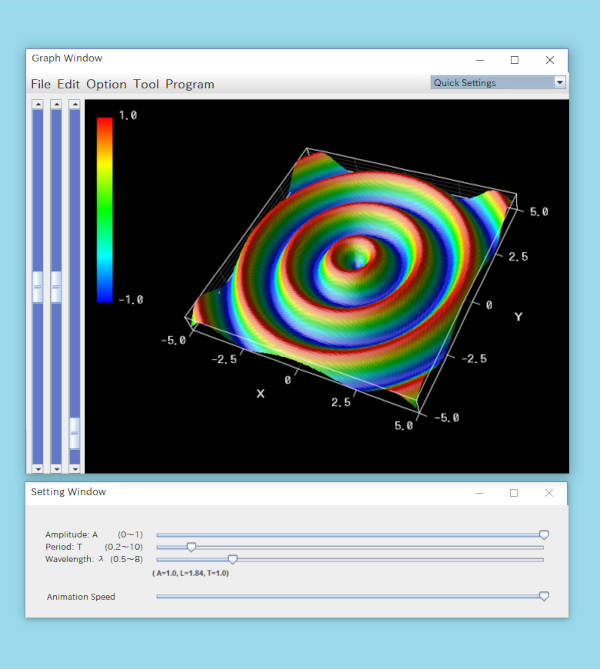
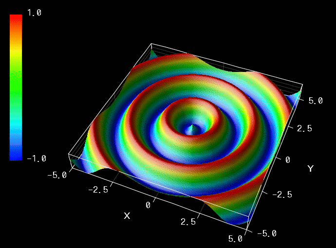
In the graph window, you'll see an animated circular wave spreading out. The parameter setting window allows you to control the wave's properties, such as wavelength, amplitude, and period, using sliders.

Closing either window will terminate the program.

Concept Overview

A circular wave occurs when a vibrating source, known as the wave source, transfers its motion outward through the surrounding medium in concentric circles.

If you gently touch the surface of water -- say, in a bathtub -- you'll observe waves radiating outward in a circular shape.

And if you vibrate your finger vertically against the surface, concentric wavefronts will continue to propagate outward. (In that case, your finger acts as the wave source.)

To simplify this motion, let's assume the following:

Now, if the wave source performs a simple harmonic motion, this movement propagates outward with delay proportional to distance.

As a result, if you take a cross-section of the wave in the radial direction, what you'll see is a classic sine wave -- just like the one we examined in the first article of this series.

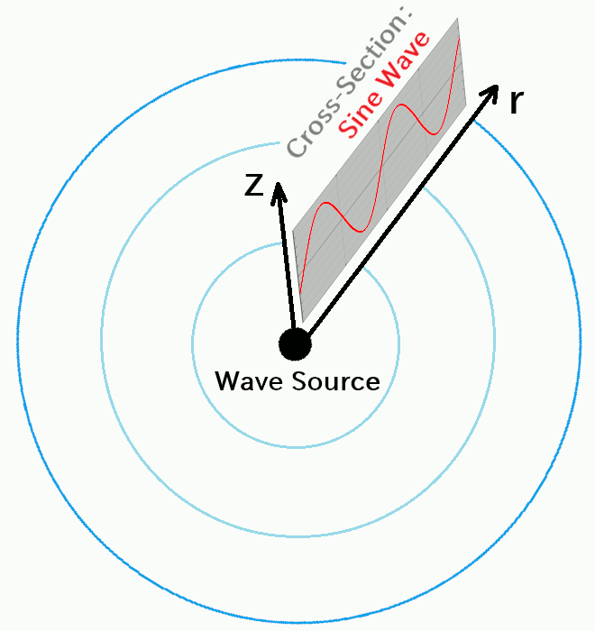
We define the direction of oscillation -- that is, the direction in which the wave source moves up and down -- as the \(z\)-axis, and the horizontal distance from the wave source as \(r\).

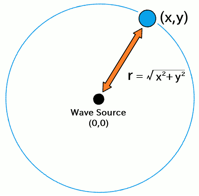
Assuming the wave source is located at the origin of the coordinate system, the distance \(r\) from the wave source to a point \((x,y)\) on the surface is given by:

\[ r = \sqrt{x^2 + y^2} \tag{1}\]

Here's how it looks geometrically:

To express the motion mathematically, we can now rewrite the horizontal variable \(x\) in the sine wave equation from the earlier article as \(r\), to obtain a formula for a sine wave that propagates radially from the source:

\[ z = A \sin 2 \pi \bigg( \frac{t}{T} - \frac{r}{\lambda} \bigg) \tag{2} \]

This is the mathematical expression for the circular wave shown in the animation. It's a simplified theoretical model that is easy to work with and is often used in introductory explanations of wave interference.

Here, \(A\) is the amplitude, \(\lambda\) the wavelength, and \(T\) the period -- all of which were introduced in this earlier article, so please refer back to that for more detail.

Code Overview

This program is written in VCSSL.

Let's go over the contents of the code briefly. VCSSL has a simple C-like syntax, so if you've had any exposure to C or similar languages, you should find it easy to follow.

If you'd like to customize things -- such as the graph's range or other behavior -- just open the program file, CircularWave.vcssl, in a text editor and modify it freely. Since VCSSL is a scripting language, there's no need for a separate compiler or build step -- just save your changes and run.

Full Code

Let's start by looking at the entire code:

That's it! The program is just under 250 lines long.

Each section is explained in the comments within the code itself, but let's go over a few key parts in more detail, especially those that differ from the sine wave animation program two articles ago.

The overall structure is nearly identical to the previous version -- the only major changes are that:

• The wave data is now two-dimensional instead of one-dimensional.
• A 3D graph is used instead of a 2D graph.

If you haven't already, reviewing the previous sine wave animation article is highly recommended to understand the basics.

In this article, we'll focus on the differences from that version.

Variable Declarations

The variable declarations at the top of the code are mostly the same as before, but we've added new variables to handle the Z-direction, which wasn't needed for 1D waves.

The arrays "waveX", "waveY", and "waveZ" store the coordinates of each point on the mesh grid where the wave is defined.

In the earlier sine wave version, the wave was confined to a one-dimensional line along the X-axis, so a 1D array was sufficient.

Here, the wave exists on a 2D surface (the X-Y plane), so we use **2D arrays** to define a mesh grid of points.

The mesh consists of N grid points along both X and Y, meaning there are (N-1) intervals along each axis. The spacing of those intervals is given by "DX" and "DY", respectively.

main Function

Now let's take a look at the main() function:

This structure is also nearly identical to the earlier sine wave version.

Inside the animation loop ( "while (continuesLoop)" ), the program advances time step-by-step, calculates the wave height for each point on the 2D surface, stores it in an array, and passes the result to the 3D graph renderer.

The key part is where the wave values are calculated and stored in the arrays:

Here, the 3rd and 7th lines directly correspond to the equations (1) and (2) shown earlier in this article:

\[ r = \sqrt{x^2 + y^2} \tag{1} \] \[ z = A \sin 2 \pi \bigg( \frac{t}{T} - \frac{r}{\lambda} \bigg) \tag{2} \]

That's the equation of a circular sine wave expressed in code form.

The program works like a flipbook: it repeatedly computes equation (2) for increasing values of \(t\), sending the result to the 3D graph for animation.

This part forms the core logic of the simulation. The rest of the code is mostly concerned with building the GUI, managing the graph display, and general setup.

As for graph-related parts: VCSSL makes it easy to switch between 2D and 3D graphs using a nearly identical interface. Most of the changes are just replacing "2D" with "3D" in the function names. GUI setup and event handling also follow the same pattern as before.

License

This VCSSL/Vnano code (files with the ".vcssl" or ".vnano" extensions) is released under the CC0 license, effectively placing it in the public domain. If any sample code in C, C++, or Java is included in this article, it is also released under the same terms. You are free to use, modify, or repurpose it as you wish.

* The distribution folder also includes the VCSSL runtime environment, so you can run the program immediately after downloading. The license for the runtime is included in the gLicenseh folder.
(In short, it can be used freely for both commercial and non-commercial purposes, but the developers take no responsibility for any consequences arising from its use.) For details on the files and licenses included in the distribution folder, please refer to "ReadMe.txt".

* The Vnano runtime environment is also available as open-source, so you can embed it in other software if needed. For more information, see here.