Now Loading...

Please download on PC (not smartphone) and extract the ZIP file. Then double-click VCSSL.bat (batch file) to execute for Microsoft® Windows®, or execute VCSSL.jar (JAR file) on the command line for Linux® and other OSes.
For details, see How to Use.

Vnano | Compute Integrated Value Numerically (Numerical Integration)

An example program (script) to perform integration numerically. This script uses simpson's rule by default, but you can use the rectangular method and the trapezoidal method with modifying a line in code.

Code of this script is written in the Vnano. Code written in C, C++, and Java® are also distributed in Code section. In addition, the Vnano is a subset of the VCSSL, so you can execute this script as VCSSL code, with changing the extention of the script file to ".vcssl" (In such case, please enable the "import" statement at the near the top of the code, which is commented-out by default).

Also, if you want to plot the graph of the integrated function, see the next article and code.

Sponsored Link

How to Use

Download and Extract

At first, click the "Download" button at the above of the title of this page by your PC (not smartphone). A ZIP file will be downloaded.

Then, please extract the ZIP file. On general environment (Windows®, major Linux distributions, etc.), you can extract the ZIP file by selecting "Extract All" and so on from right-clicking menu.

» If the extraction of the downloaded ZIP file is stopped with security warning messages...

Execute this Program

Next, open the extracted folder and execute this VCSSL program.

For Windows

Double-click the following batch file to execute:

For Linux, etc.

Execute "VCSSL.jar" on the command-line terminal as follows:

» If the error message about non-availability of "java" command is output...

How to Use After Executing The Program

Output the Integrated Value

When the program has started, a window will be launched. Then, when the calculation has completed, a small window will be launched, and the integrated value will be displayed on it.

By default, the calculation will be completed soon. If you make the value of "N" in the script larger, required time of the calculation become longer,

How to Change the Integrant Function, Interval, etc.

For changing the integrant function, modify the content of the function "f(x)" defined in the script. For changing the interval of the integration, modify values of variables "A" and "B" in the script. In addition, if necessary, modify the value of the variable "N" in the script, which is the number of tiny intervals (See: Code section).

By default settings, "cos(x)" will be integrated from x = 0 to x = 1.

How to Change The Algorithm of the Integration

In this script, as algorithms of the numerical integration, you can use the rectangular method, the trapezoidal method, and the Simpson's rule. Each algorithm is implemented as a line in the script (See: Code section), so please add/remove "//" (a line starts with "//" will be ignored) at those lines, for selecting the algorithm you want to use. By default, the Simpson's rule will be used.

Other - How to Plot The Graph of The Integrated Function

If you want to plot the graph of the integrated function, we are destributing the modified version of this script for such purpose:

• Vnano | Output Data for Plotting The Graph of The Integrant Function

In the above article, we are explaining how to plot the output data into a graph.

Code and Algorithms

Entier Code

Code of this program is written in the Vnano. The Vnano has a simple C-like syntax, so if you accustomed with C or C-like programming languages, you probably can read/customize the content of code easily.

Let's see the entier code:

The Top of Code

Code starts with the following content:

The first line "coding ..." is for declaring the text-encoding of the script file, for preventing encoding/decoding-related probrems (e.g.: "mojibake").

The next line "import ..." (which is used for loading a library) is necessary if you execute this script as VCSSL code, but it is not necessary when you exeute this script as Vnano code, so it is commented-out by default.

Definitions of The Integrant Function, The Interval of The Integration, etc.

In the next part, the integrant function, the interval of the integration, and so on are defined:

When you want to customize settings of the integration, modify the above code. Basically, define the integrant function as the function "f(x)" in the above code, and input the value of the lower/upper-limit of the integration to the variable "A" / "B".

"N" represents the number of tiny intervals (for details, see the latter sections). When you make the value of N larger, the precision of the integrated value basically increses, but required time for the calculation become longer. Please note that, if you set the immediately large value to N, the precision might decrease, because the number of total cycles of the integration loop become very large, so tiny numerical errors affect many times to the result.

The Core Part: Performing The Numerical Integration

The next part is, the core part of this script performing the numerical integration:

If you read the above code without any background knowledge, you might not be able to understand meanings of comments in the above code, but don't worry. Let's see keypoints of numerical integration algorithms briefly and graphically.

Calculate The Value of The Integration By Counting-Up Area Numerically

There are many kind of numerical integration algorithms in the world, but three methods used in this script are based on a common concept: calculate the value of the integration by numerically counting-up area between the integrant function f(x) and x-axis:

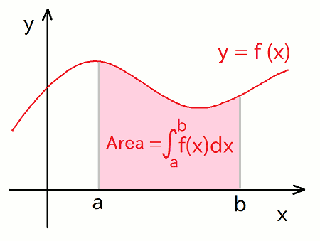
The area painted by the red color in the above figure equals to the integrated value of  f(x) from a to b.

Why? What condition is assumed? It is difficult to answer those questions strictly. It requires some complicated mathematical discussions about definitions of integral and integrability.

We don't want to discuss about it here, so, Let's assume that we choose a standard (not trickey, ���[�}�� integrable) function as the integrant function f(x), and then the area of the above figure equals to the integrated value.

Rectangular Method

As mentioned above, our goal is very simple: we want to calculate the area painted by the red color in the above figure, as precise as possible. Let's discuss how calculate the area in programs.

Probably the most simple way is as follows: Firstly split the entier area into N-"tiny interval"s, and then approximate the value of area of each tiny interval as a rectangle of which height is the value of  f(x) at the left-bottom of the tiny area, and finally calculate the summation value of area of all rectangles (see the following figure).

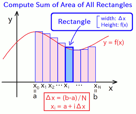
This is so-called "the rectangular method".

Does it make sense? Let's return to code. You can use the rectangular method by removing "//" from the head of the line of the rectangular method, and adding "//" to the head of the line of the Simpson's rule. Then, with removing unnecessary lines, code become as follows:

In the above code, the left-hand-side of the last line "f(x) * delta" represents area of a rectangle of a tiny interval. The above code calculates the summation value of it of all rectangles with moving the value of x in the for-loop.

By the way, by default settings, this script calculated the integrated value of cos(x) from 0 to 1, so the theoretically correct value is sin(1) = 0.8414709848078965... . On the other hand, the numerically integrated value depends on the value of N. The followings are results by using the rectangular method:

As the above, with making the value of N larger, we can get more precise result. More strictly, when we make the value of N about 1 digit (10 times) larger, the length of correct digits in the result increases about 1 digit.

Trapezoidal Method

Errors between the correct value and calculated values by using the rectangular method are mainly caused by that: we has approximated the value of area between the x-axis and the "roundy curve" of  f(x) by using "edgy rectangles".

Hence, as the next step, Let's approximate the curve of  f(x) by using a polyline of which nodes are \( (x,y) = (x_i, f(x_i)) \), where \(x_i\) is the x-coordinate value of the left-bottom point of i-th tiny interval (i = 0, 1, 2, ..., N-1) :

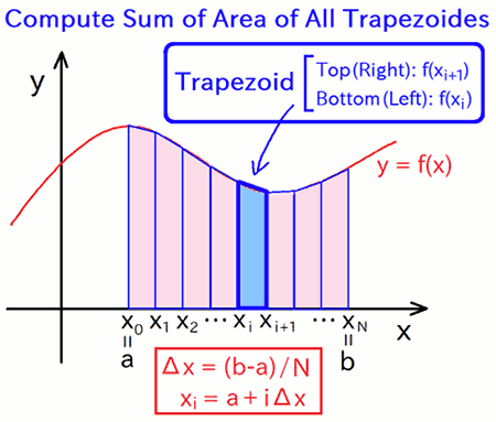
By the above improvement of the approximation, rectangles of the rectangular method become trapezoides. This is so-called "the trapezoidal method".

You can use the trapezoidal method by removing "//" from the head of the line of the trapezoidal method, and adding "//" to the head of the line of the Simpson's rule. Then, with removing unnecessary lines, code become as follows:

In the above code, the left-hand-side of the last line "( f(x) + f(x+delta) ) * delta / 2.0" represents area of a trapezoid of a tiny interval. The above code calculates the summation value of it of all trapezoides with moving the value of x in the for-loop.

Calculation results by using the trapezoidal method, under the same settings with the rectangular method, are followings:

As the above, when we make the value of N about 1 digit (10 times) larger, the length of correct digits in the result increases about 2 digits. In the contrast, when we used the rectangular method, we were required to make the value of N about 100 times larger, for improving the precision about 2 digits.

Simpson's Rule

Let's continue to improve the approximation. In the trapezoidal method, we have approximated the curve of  f(x) in a tiny interval by using a line, as depicted in the following figure:

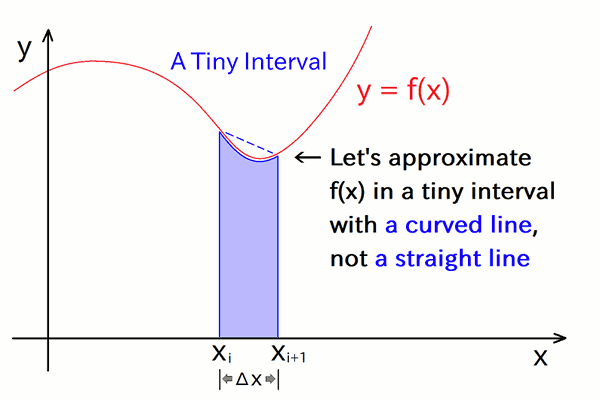
As commented in the above figure, in a tiny interval, if we can approximate f(x) by using a manually integrable curve which fits with f(x) well, its integrated value gives more good approximation of area of a tiny interval, than a trapezoid.

Hence, Let's approximate f(x) in a tiny interval by using a quadratic function throughing same points as f(x), at both-side boundaries and the center of the tiny interval:

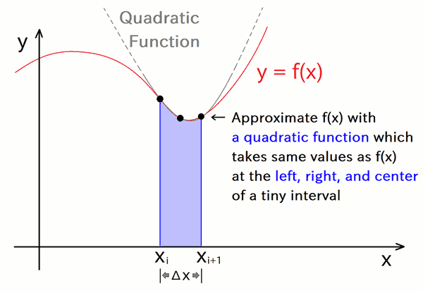
In general, parameters of a n-dimentional polynomial equation can be determined when values at (n + 1) points are given, so parameters of the above quadratic (2-dimentional) function can be determined, because values at (2 + 1) points are given. Then, we can calculate the integrated value of the determined quadratic function manually.

The result of the above calculation is well-known as the Simpson's rule. By using the Simpson's rule, we can get the approximate value of the area of i-th tiny interval, \(A_i\), as follows:

\[ A_{i} = \frac{ f(x_i) + f(x_i + \Delta x) + 4f(x_i+ \Delta x / 2) }{6} \Delta x \]

As the rectangular method and trapezoidal method, calculate the summation of \(A_i\) for all i ( = 0, 1, 2, ..., N-1).

This script uses the Simpson's rule by default. With removing unnecessary lines, code calculating area by using the Simpson's rule are as follows:

In the above code, the left-hand-side of the last line "( f(x) + f(x+delta) + 4.0 * f(x+delta/2.0) ) * delta / 6.0" represents an approximate value of area of a tiny interval \(A_i\). The above code calculates the summation value of it of all \(A_i\) with moving the value of \(x (= x_i)\) in the for-loop.

Let's check the precision:

As the above, when we make the value of N about 1 digit (10 times) larger, the length of correct digits in the result increases about 4 digits. In the contrast, when we used the rectangular method, we were required to make the value of N about 10000 times larger(!!!), for improving the precision about 4 digits. Even when we used the trapezoidal method, it required to make N 100 times larger.

Also, as we can recognize in above results, please note that we can NOT improve the precision of the result beyond the limit of the numerical data type used for calculations (in this script/article, we have used "64-bit binaly floating-point number"). If you forget the above thing, and if you set the value of N to an immediately large number, the precision goes lower than the best, because the number of total cycles of the integration loop become very large, so tiny numerical errors affect many times to the result. The best value of N depends on f(x) and the interval of the integration, so check the behaviour of results with changing the value of N, as we did in this article.

License

The license of this VCSSL / Vnano code (the file with the extension ".vcssl" / ".vnano") is CC0 (Public Domain), so you can customize / divert / redistribute this VCSSL code freely.

Also, if example code written in C/C++/Java are displayed/distributed on Code section of this page, they also are distributed under CC0, unless otherwise noted.