Controlling the Origin Position of a Coordinate System

So far, we've covered how to move coordinate systems by applying incremental displacements relative to their current positions. However, in some cases, you may want to directly specify the position of a coordinate system's origin. This section explains how to do that.

Direct Control of the Origin Position

Setting the Origin Position

To directly set the origin position of a coordinate system, use the setCoordinateLocation(...) function.

- Function Format -

Arguments:

• coordinateID: The ID of the coordinate system to modify.
• x, y, z: The X, Y, and Z components of the desired origin position.

Getting the Origin Position

To retrieve the origin position of a coordinate system, use the getCoordinateLocation(...) function.

- Function Format -

The "coordinateID" argument specifies the target coordinate system.

The return value is an array in which:

• [0] holds the X component,
• [1] holds the Y component,
• [2] holds the Z component

of the origin position.

Example Program

Let's try placing a local coordinate system on top of the world coordinate system, and moving it by directly setting its origin position to follow an animated path.

To make the systems easier to distinguish, a smaller axis model is mounted on the local coordinate system, while a larger one is mounted on the world coordinate system.

import graphics3d.Graphics3DFramework;
import Graphics3D;
import Math;  // For using the sin function


// Variable to hold the coordinate system ID
int coord;

// Time counter (in update cycles)
int t = 0;


// Function called at the start of the program
void onStart ( int rendererID ) {

	// Optional screen size and background color settings
	setWindowSize( 800, 600 );
	setBackgroundColor( 0, 0, 0, 255 );


	//  Create a local coordinate system
	coord = newCoordinate( );

	// Mount it on the world coordinate system
	mountCoordinate( coord, rendererID );

	// Place a small axis model on the local coordinate system
	int axis1 = newAxisModel( 1.5, 1.5, 1.5 );
	mountModel( axis1, rendererID, coord );

	// Place a large axis model on the world coordinate system
	int axis2 = newAxisModel( 3.0, 3.0, 3.0 );
	mountModel( axis2, rendererID );
}


// Function called several times per second to update the display
void onUpdate ( int rendererID ) {

	// Move along a Lissajous curve and increment time
	setCoordinateLocation( coord, sin(0.1*t), sin(0.5*t), 0.0 );
	t++;
}

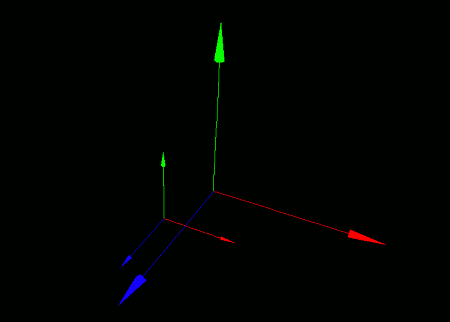
When you run this program, you'll see two axis models on a black screen.

The larger one is mounted on the world coordinate system, while the smaller one is mounted on the local coordinate system. The local coordinate system moves in a complex path, drawing a Lissajous curve.

Execution Result

A large and a small axis model appear. The small coordinate system moves in an animated pattern.